How to Detect Hidden Target Leakage in Public Datasets with Python and a Dependency Graph

Some time ago, I gave a machine learning model five columns from a public CDC dataset and asked it to predict a sixth column from the same file. The model scored an R² of 0.998, which is about as close to perfect as a real model gets.

That score looked like a success, but the model had learned very little about the real world. CDC had calculated the sixth column from the other five, so the model simply worked out CDC’s formula.

Data scientists call this problem target leakage, and it happens when the inputs you give a model already contain the answer in some form.

Leakage like this hides easily in public data, because a large share of public data is calculated from other public data. A government index might be built from survey columns, and a second index might be built from the first one. Agencies explain these recipes in their methodology PDFs, yet data catalogues rarely store them in a form a computer can check.

In this tutorial, you’ll write that record yourself and then build a small Python tool that reads it. The tool works like the dependency checker inside a package manager: you tell it what you want to predict and which columns you plan to use, and it refuses any column that sits on a derivation path to or from your target.

By the end, you’ll know how to:

• reproduce a real leak using live CDC data and scikit-learn

• describe what a dataset was built from in a small YAML file called a manifest

• walk that graph with breadth-first search and depth-first search

• make a checking tool that fails loudly on typos, broken files, and empty inputs

• run the check automatically on every push with GitHub Actions

Table of Contents

Prerequisites

To follow along, you’ll need:

• Python 3.10 or newer

• a basic idea of what a pandas DataFrame is

• a terminal where you can run commands

• about 7 MB of free disk space for the CDC data file

Create a fresh project folder with a virtual environment inside it, so these libraries stay separate from the rest of your system. Then install the three libraries this tutorial uses:

mkdir leak-tutorial
cd leak-tutorial
python3 -m venv .venv
source .venv/bin/activate
pip install pandas scikit-learn pyyaml

On Windows, run .venv\Scripts\activate in place of the source line, and type python wherever this article says python3. Run every command in this tutorial from inside the leak-tutorial folder.

Every file you build in this tutorial is also in the companion repository, derives-from-tutorial, so you can compare your work against it if you get stuck.

The full version of the tool lives in a public GitHub repository, and I link to it at the end of the article.

Key Terms in Plain English

Here are five words that come up again and again in this tutorial:

• Target: the column you want your model to predict.

• Covariate: a column you feed into the model to help it predict the target (many people call these features).

• R² (R-squared): a score that tells you how closely a model’s predictions match the real values. A score of 1.0 means a perfect match, and a score near 0 means the model explains very little.

• Census tract: a small area of the United States that usually holds about 4,000 people, roughly the size of a neighbourhood.

• Cross-validation: a fair way to test a model. You split the data into five parts, train on four, test on the fifth, and repeat until every part has had a turn as the test set.

Step 1: See the Leak for Yourself

The US Centers for Disease Control and Prevention (CDC) publishes the Social Vulnerability Index, or SVI. Emergency planners use it to find communities that may need extra help during a flood, a heatwave, or a disease outbreak.

CDC builds the SVI in layers. It starts with 16 columns from the American Community Survey (ACS), a large survey run by the US Census Bureau. Each column is a percentage, such as the share of people living in poverty or the share of households with zero vehicles.

CDC groups those 16 columns into four themes and ranks every census tract within each theme. It then combines the four theme ranks into one overall rank called RPL_THEMES.

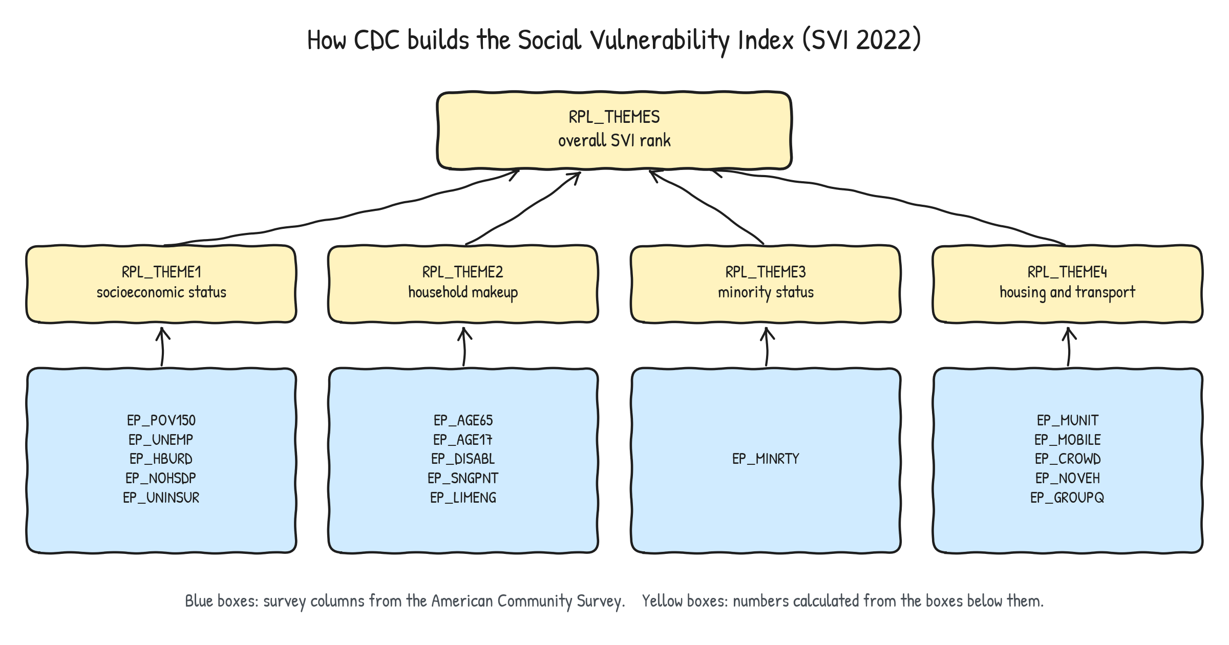
How CDC builds the SVI: 16 ACS survey columns feed four theme ranks, and the four theme ranks feed the one overall rank. Every yellow box is calculated from the boxes below it.

Here’s the detail that matters for this tutorial: CDC ships the raw ACS columns and the finished ranks together in the same CSV file. That makes it very easy to grab both and put them into one model.

Download the California file:

curl -L -o California.csv https://svi.cdc.gov/Documents/Data/2022/csv/states/California.csv

I use curl here because some Python installs on macOS fail to verify the website’s security certificate when they download files directly.

Now create a file called leak_demo.py:

"""leak_demo.py: predict a published index from the columns it was built from."""
import pandas as pd
from sklearn.ensemble import HistGradientBoostingRegressor
from sklearn.model_selection import KFold, cross_val_score

# CDC marks missing values as -999, so turn those into proper blanks.
df = pd.read_csv("California.csv", low_memory=False).replace(-999, float("nan"))


def score(inputs, target):
    data = df[inputs + [target]].dropna()
    model = HistGradientBoostingRegressor(random_state=0)
    folds = KFold(n_splits=5, shuffle=True, random_state=0)
    r2 = cross_val_score(model, data[inputs], data[target],
                         cv=folds, scoring="r2").mean()
    print(f"{target:<11} from {len(inputs)} column(s)  "
          f"tracts={len(data)}  R2 = {r2:.3f}")


# Theme 1 is built from exactly these five columns.
score(["EP_POV150", "EP_UNEMP", "EP_HBURD", "EP_NOHSDP", "EP_UNINSUR"],
      "RPL_THEME1")

# EP_NOINT ships in the same file, and CDC leaves it out of the index.
score(["EP_NOINT"], "RPL_THEMES")

Here’s what the script does:

1. It loads the CSV and turns CDC’s -999 markers into blank values, because CDC uses -999 to flag a missing value.

2. The score function trains a gradient boosting model, which is a strong and popular choice for tables of numbers, and it measures R² with five-fold cross-validation.

3. The first call predicts Theme 1 using the exact five columns CDC used to build Theme 1.

4. The second call predicts the overall rank using EP_NOINT, the share of households lacking a broadband internet subscription. CDC includes this column in the same file and leaves it out of the index.

Run it:

python3 leak_demo.py

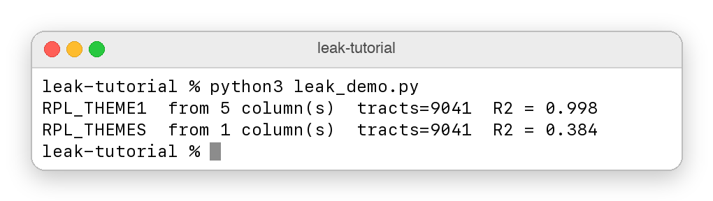
The output of leak_demo.py. Theme 1, predicted from the five columns CDC built it from, scores R² = 0.998. The overall rank, predicted from a column CDC leaves out of the index, scores 0.384.

The first score is 0.998, which means the model rebuilt CDC’s Theme 1 almost perfectly. CDC’s formula is a fixed recipe, and the model had every ingredient.

The second score is 0.384. EP_NOINT sits beside the index in the file, and its score shows the size of an ordinary link between two related measures.

Now imagine a paper that reports R² = 0.998 for predicting social vulnerability. That number would look like a breakthrough, yet it would only show that the model had found CDC’s recipe.

The scores in this article came from scikit-learn 1.8.0. They stay the same to three decimal places across scikit-learn 1.3.2 to 1.9.0, so your run should match.

Step 2: Understand Why Public Data Leaks

The SVI example is easy to spot because the inputs and the index sit in one file. Most real cases are harder, because the chain runs across several agencies.

Here’s one real chain that crosses three organisations. FEMA’s National Risk Index (NRI) includes a social vulnerability score. According to FEMA’s technical documentation (version 1.20, December 2025), that score comes from the Census Bureau’s Community Resilience Estimates. The Census Bureau builds those estimates from ACS survey data.

So a FEMA risk score and an ACS column can sit at two ends of one chain, even though they come from different agencies and different websites.

To see why computers miss this, you need to know about two kinds of history a number can have:

• Provenance answers the question “Where did this number arrive from?” For example, a value came from California.csv, which came from svi.cdc.gov.

• Derivation answers the question “What was this number calculated from?” For example, Theme 1 was calculated from five ACS columns.

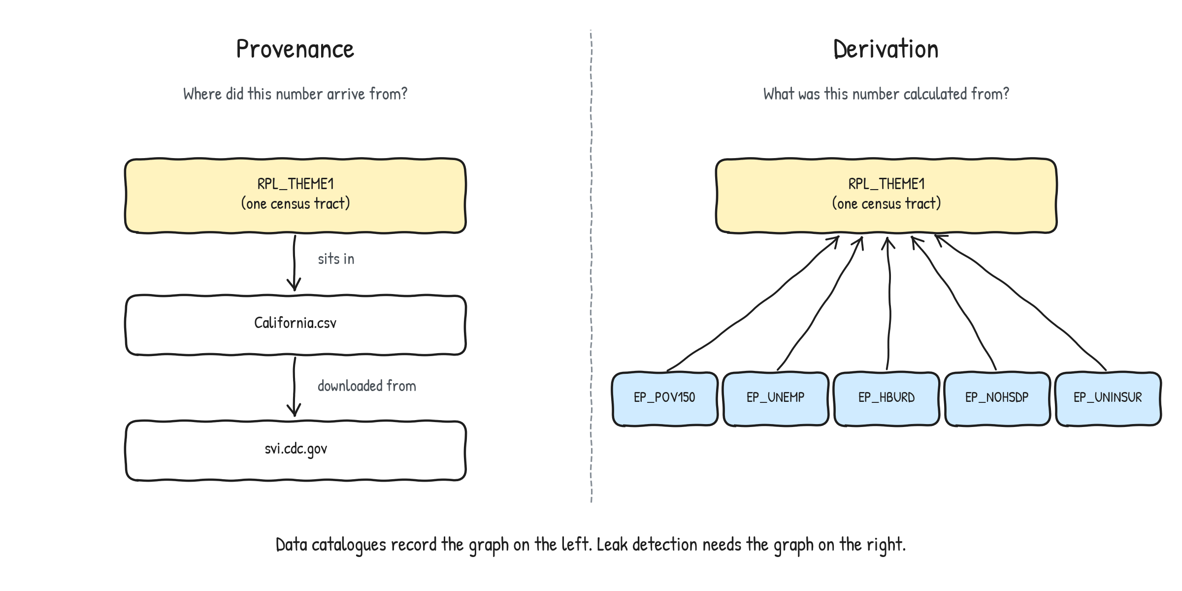
Two kinds of history a number can have. Provenance, on the left, records the file and the website a value arrived from. Derivation, on the right, records the five ACS columns Theme 1 was calculated from.

Most data catalogues store provenance well, and Google’s Data Commons is a good example: it defines provenance as “the physical unit of an import”, which tells you the file a number came in. Derivation usually lives only in PDF methodology documents written for humans.

So when an automated pipeline searches for helpful covariates, it can happily collect columns that the target was built from. The pipeline sees high scores and keeps those columns.

Step 3: Borrow an Idea from Package Managers

Software developers solved a very similar problem long ago.

When you run pip install requests, pip reads a list of what requests depends on, then what those packages depend on, and so on down the tree. Because every dependency is written down, pip can spot trouble anywhere in the tree before it installs anything.

The diagram below puts that tree beside the data version of the same problem.

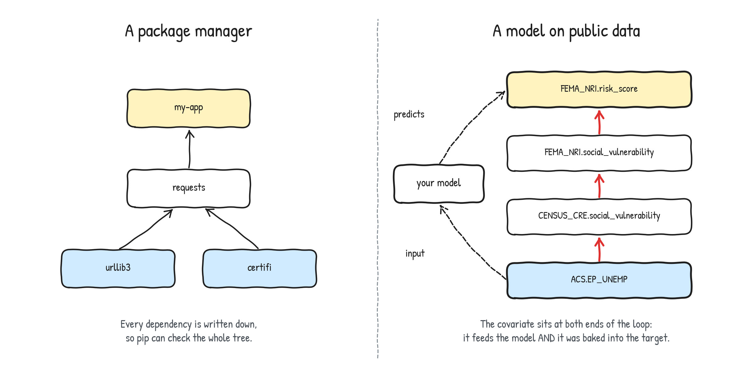
The same shape twice. On the left, pip’s dependency tree: urllib3 and certifi feed requests, which feeds my-app. On the right, the data version: ACS.EP_UNEMP goes into a model that predicts FEMA_NRI.risk_score, and the same column also climbs through two other products into that risk score.

Public data needs the same kind of record. In the right-hand half of the diagram above, ACS.EP_UNEMP (the unemployment rate) goes into the model as a covariate. The same column also climbs up through two other products into FEMA_NRI.risk_score, which is the target. The column sits at both ends of the loop.

In computer science, this kind of diagram is a graph. Each box is a node, and each arrow is an edge. In a data graph, following the arrows always leads you upward and away from where you started, so the graph is a directed acyclic graph, or DAG for short. “Acyclic” means the arrows form zero loops.

Throughout this article, every arrow points from an ingredient to the product made from it.

Two family words help describe positions in the graph:

• An ancestor of a node is anything you reach by following arrows backwards from it, at any distance. The ACS columns are ancestors of the SVI.

• A descendant of a node is anything you reach by following arrows forwards from it. The SVI is a descendant of the ACS columns.

Your leak check then becomes one simple rule: every covariate must stay clear of the target’s ancestors and descendants.

Step 4: Write the Dependency Manifest

A manifest is a file that lists every product and what each one was built from. You’ll use YAML here because people can read and edit it easily.

Here’s how one measured product looks:

ACS.EP_UNEMP:
  label: Unemployment rate
  measurementBasis: measured
  derivesFrom: []

The empty list in derivesFrom: [] records zero parents, because this product comes straight from a survey.

And here is a product built from another product:

FEMA_NRI.social_vulnerability:
  label: FEMA National Risk Index, social vulnerability
  measurementBasis: composite
  derivesFrom:
    - {variable: CENSUS_CRE.social_vulnerability, relation: identity, confidence: documented}

Each entry in derivesFrom is one edge in the graph, and every edge carries three facts:

• variable holds the name of the parent product, and that name must match a product defined elsewhere in the file.

• relation describes how the parent was used.

• confidence records how sure you are about the edge.

These are the five relations:

relation	meaning
component	the parent is a mathematical ingredient, like one number in a sum
modelled_from	the parent was an input to a statistical model
identity	the product is the parent, republished under a new name
poststratified_on	the parent supplied the population weights
denominator	the parent is the bottom number of a fraction, like population in “cases per person”

These are the three confidence levels:

confidence	meaning
certain	the formula is published, or the inputs and outputs ship together in one file
documented	the agency states the link in its own methodology document
inferred	the documents strongly imply the link, so treat it as provisional

The confidence field matters more than it first appears. A lineage graph full of guesses would recreate the same problem it aims to solve, so each edge should say how much evidence stands behind it.

Each product also has a measurementBasis:

measurementBasis	meaning
measured	counted or surveyed directly, like a census count
modelled	produced by a statistical or machine learning model
composite	calculated with fixed arithmetic from other products

This field records something public catalogues usually leave out: whether a number was counted or predicted. A census count and a random forest prediction look identical in a spreadsheet, yet they’re very different kinds of evidence.

Now create mini-manifest.yaml with the content below. It’s a trimmed slice of the full manifest with 11 products from real US data infrastructure, and each product keeps a few of its real edges so the file stays short.

# A small slice of derivation-manifest.yaml, used in the tutorial.
schema: derives-from/0.2

products:

  # ---- measured: counted or surveyed directly
  ACS.EP_POV150:
    label: Population below 150% of the poverty line
    measurementBasis: measured
    derivesFrom: []

  ACS.EP_UNEMP:
    label: Unemployment rate
    measurementBasis: measured
    derivesFrom: []

  ACS.EP_NOVEH:
    label: Households with zero vehicles
    measurementBasis: measured
    derivesFrom: []

  SAT.chirps_rainfall:
    label: CHIRPS satellite rainfall
    measurementBasis: measured
    derivesFrom: []

  NVSS.mortality:
    label: Death certificate records
    measurementBasis: measured
    derivesFrom: []

  # ---- built from other products
  CENSUS_CRE.social_vulnerability:
    label: Census Community Resilience Estimates, social vulnerability
    measurementBasis: modelled
    derivesFrom:
      - {variable: ACS.EP_POV150, relation: modelled_from, confidence: documented}
      - {variable: ACS.EP_UNEMP,  relation: modelled_from, confidence: documented}
      - {variable: ACS.EP_NOVEH,  relation: modelled_from, confidence: documented}

  FEMA_NRI.social_vulnerability:
    label: FEMA National Risk Index, social vulnerability
    measurementBasis: composite
    derivesFrom:
      - {variable: CENSUS_CRE.social_vulnerability, relation: identity, confidence: documented}

  HVRI.bric:
    label: Baseline Resilience Indicators for Communities
    measurementBasis: composite
    derivesFrom:
      - {variable: ACS.EP_UNEMP, relation: component, confidence: documented}
      - {variable: ACS.EP_NOVEH, relation: component, confidence: documented}

  FEMA_NRI.community_resilience:
    label: FEMA National Risk Index, community resilience
    measurementBasis: composite
    derivesFrom:
      - {variable: HVRI.bric, relation: identity, confidence: documented}

  FEMA_NRI.expected_annual_loss:
    label: FEMA National Risk Index, expected annual loss
    measurementBasis: modelled
    derivesFrom: []

  FEMA_NRI.risk_score:
    label: FEMA National Risk Index, overall risk score
    measurementBasis: composite
    derivesFrom:
      - {variable: FEMA_NRI.expected_annual_loss, relation: component, confidence: certain}
      - {variable: FEMA_NRI.social_vulnerability, relation: component, confidence: certain}
      - {variable: FEMA_NRI.community_resilience, relation: component, confidence: certain}

Step 5: Build the Linter

A linter is a tool that reads something and warns you about problems before they cause harm. Code linters such as Flake8 read source code, while this linter reads your manifest and your list of covariates.

Create a file called mini_lint.py. You’ll build it in six parts, and the finished file stays under 200 lines.

Part 1: Load YAML and Refuse Duplicate Keys

"""mini_lint.py: refuse covariates that sit on a derivation path to or from the target."""
import argparse
import sys
from collections import deque
from itertools import combinations

import yaml

RANK = {"certain": 3, "documented": 2, "inferred": 1}
DETERMINISTIC = {"component", "identity", "denominator"}


def fail(message):
    """Exit code 2 means the manifest or the command itself is broken."""
    print(message, file=sys.stderr)
    sys.exit(2)


# ---------------------------------------------------------------- step 1
class StrictLoader(yaml.SafeLoader):
    """A YAML loader that stops on a repeated key."""


def refuse_duplicates(loader, node, deep=False):
    seen = {}
    for key_node, _ in node.value:
        key = loader.construct_object(key_node, deep=deep)
        line = key_node.start_mark.line + 1
        if key in seen:
            fail(f"manifest error: key {key!r} appears twice "
                 f"(line {seen[key]} and line {line})")
        seen[key] = line
    return loader.construct_mapping(node, deep=deep)


StrictLoader.add_constructor(
    yaml.resolver.BaseResolver.DEFAULT_MAPPING_TAG, refuse_duplicates)

RANK turns confidence words into numbers, so the tool can find the weakest edge in a route. DETERMINISTIC lists the relations that are pure arithmetic.

fail prints a message and exits with code 2. Later in the tutorial, you’ll see why code 2 must stay separate from code 1.

The loader deals with a sneaky YAML behaviour. If a key appears twice in the same block, PyYAML quietly keeps the last copy and throws the first one away. In a manifest, that can erase every edge of a product, and the tool would then see zero routes and happily clear a leaky covariate.

refuse_duplicates runs every time PyYAML builds a mapping (a Python dictionary). It walks through the keys, remembers the line number of each one, and stops the program as soon as a key repeats.

Part 2: Read Products and Edges

# ---------------------------------------------------------------- step 2
def load(path):
    try:
        with open(path) as fh:
            products = yaml.load(fh, StrictLoader)["products"]
    except (OSError, yaml.YAMLError, KeyError, TypeError) as e:
        fail(f"manifest error: unable to read {path}: {e}")

    edges = {}
    for name, product in products.items():
        edges[name] = []
        for e in product.get("derivesFrom") or []:
            if RANK.get(e.get("confidence")) is None:
                fail(f"manifest error: {name} has an edge with "
                     f"confidence {e.get('confidence')!r}")
            edges[name].append((e["variable"], e["relation"], e["confidence"]))
    return products, edges

load opens the file with the strict loader. If anything goes wrong while reading, such as a bad path or broken YAML, it calls fail.

It then builds a dictionary called edges. For each product name, it stores a list of (parent, relation, confidence) tuples. For example:

edges["FEMA_NRI.social_vulnerability"]
# [("CENSUS_CRE.social_vulnerability", "identity", "documented")]

It also checks that every confidence value is one of the three allowed words. A typo such as documneted would otherwise slip through and break the ranking later.

Part 3: Check the Manifest Before Trusting It

# ---------------------------------------------------------------- step 3
def undefined_names(products, edges):
    mentioned = {parent for rows in edges.values() for parent, _, _ in rows}
    return sorted(mentioned - set(products))


def find_cycle(edges):
    state = {}

    def visit(node, stack):
        state[node] = "open"
        stack.append(node)
        for parent, _, _ in edges.get(node, []):
            if state.get(parent) == "open":
                return stack[stack.index(parent):] + [parent]
            if parent in state:
                continue
            cycle = visit(parent, stack)
            if cycle:
                return cycle
        stack.pop()
        state[node] = "closed"
        return None

    for node in edges:
        if node in state:
            continue
        cycle = visit(node, [])
        if cycle:
            return cycle
    return None

A typo in a parent name, such as HVRI.brick in place of HVRI.bric, creates an edge that points at a product the file lacks. The traversal would stop at that dead end, and every covariate beyond it would look safe.

undefined_names collects every parent mentioned in any edge and subtracts the set of defined products. Anything left over is either a typo or a product you forgot to add.

find_cycle makes sure the manifest really is a DAG. A product built from itself is impossible in real data, and a loop would send the route finder around in circles forever.

The function uses depth-first search with two labels. When the search enters a node, it marks that node open. When it has finished exploring everything above the node, it marks it closed. If the search reaches a node that’s still open, it has walked in a circle, and the function returns that circle so you can see it.

Part 4: Walk the Graph

# ---------------------------------------------------------------- step 4
def ancestors(edges, node):
    """Every product that `node` was built from, at any distance."""
    found = set()
    queue = deque([node])
    while queue:
        current = queue.popleft()
        for parent, _, _ in edges.get(current, []):
            if parent in found:
                continue
            found.add(parent)
            queue.append(parent)
    return found


def routes(edges, start, goal):
    """Every path from start up to goal. Safe because step 3 ruled out cycles."""
    found = []
    for parent, relation, confidence in edges.get(start, []):
        step = (parent, relation, confidence)
        if parent == goal:
            found.append([step])
        else:
            for rest in routes(edges, parent, goal):
                found.append([step] + rest)
    return found


def describe(start, route):
    chain = " -> ".join([start] + [parent for parent, _, _ in route])
    weakest = min(route, key=lambda step: RANK[step[2]])[2]
    arithmetic = all(rel in DETERMINISTIC for _, rel, _ in route)
    kind = "deterministic" if arithmetic else "statistical"
    return [chain, f"{kind}, weakest link: {weakest}"]

ancestors uses breadth-first search (BFS), so picture a queue at a ticket counter: you put the starting product in the queue. On each turn, you take the product at the front, look up its parents, and add each parent you have yet to see to the back of the queue. When the queue is empty, the found set holds every ancestor at every distance.

The found set also stops the search from visiting the same product twice. That matters because many products share parents.

ancestors tells you whether a covariate is upstream, and routes tells you how it gets there.

routes uses depth-first search with recursion. For each parent of start, it checks whether that parent is the goal. If it is, that single step is a complete route. Otherwise, the function calls itself to find every route from the parent to the goal, then puts the current step on the front of each one.

The function returns every route, and that choice is deliberate. An earlier version of my full tool reported only the shortest route, so the report showed whichever route had the fewest hops, even when a longer route rested on stronger evidence.

The recursion is safe here only because Part 3 already confirmed that the graph is a DAG.

describe turns a route into two readable lines. The first line is the chain of names. The second line says whether the route is deterministic (arithmetic at every step) or statistical (at least one model in the chain), and it names the weakest confidence level along the route, since a chain is only as strong as its weakest link.

Part 5: The Audit

The audit looks for three shapes in the graph:

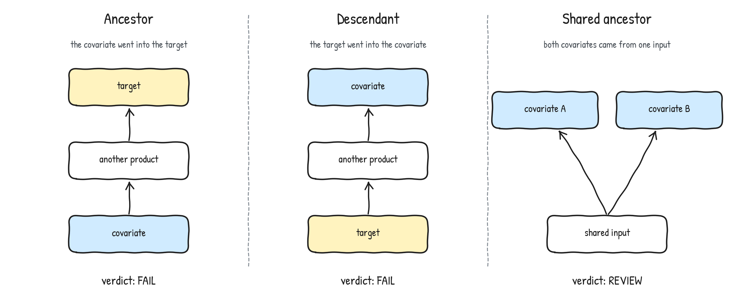
Each panel shows one shape and the verdict it produces: an arrow running into the target (FAIL), an arrow running out of the target (FAIL), and two covariates hanging off one shared input (REVIEW).

• Ancestor: the covariate went into the target, directly or through other products. This is the classic leak, so the tool reports it as an error.

• Descendant: the target went into the covariate. Predicting a parent from its own child leaks just as badly, so this is also an error.

• Shared ancestor: two covariates came from the same input. This is a softer problem, because the pair carries overlapping information, so the tool raises a warning for a person to review.

# ---------------------------------------------------------------- step 5
def audit(products, edges, target, covariates):
    findings = []

    unknown = [n for n in [target, *covariates] if products.get(n) is None]
    if unknown:
        return [("ERROR", f"unknown name: {n}", ["check the spelling"])
                for n in unknown]

    target_ancestors = ancestors(edges, target)
    for cov in covariates:
        if cov in target_ancestors:
            found = routes(edges, target, cov)
            details = [line for r in found for line in describe(target, r)]
            findings.append(("ERROR", f"{cov} is an ancestor of the target "
                                      f"({len(found)} route(s))", details))
        if target in ancestors(edges, cov):
            found = routes(edges, cov, target)
            details = [line for r in found for line in describe(cov, r)]
            findings.append(("ERROR", f"{cov} is a descendant of the target "
                                      f"({len(found)} route(s))", details))

    for a, b in combinations(covariates, 2):
        if a in ancestors(edges, b) or b in ancestors(edges, a):
            findings.append(("ERROR", f"{a} and {b}: one is built from the other", []))
        elif ancestors(edges, a) & ancestors(edges, b):
            shared = sorted(ancestors(edges, a) & ancestors(edges, b))
            findings.append(("WARN", f"{a} and {b} share ancestors", shared))
    return findings

The audit starts with name checks: if you misspell a covariate, the tool reports an error straight away, because it holds zero information about a name outside the manifest, and calling that name safe would be a guess.

Next, it computes the target’s ancestors once and tests each covariate against that set. It also computes each covariate’s ancestors to see whether the target appears among them, which is how it catches descendants.

Finally, combinations from the itertools module produces every pair of covariates. If one covariate is built from the other, that’s an error. If the pair shares any ancestor, that’s a warning.

Part 6: Verdicts and Exit Codes

# ---------------------------------------------------------------- step 6
def main():
    parser = argparse.ArgumentParser()
    parser.add_argument("--manifest", default="mini-manifest.yaml")
    parser.add_argument("--target", required=True)
    parser.add_argument("--covariates", nargs="+", required=True)
    args = parser.parse_args()

    products, edges = load(args.manifest)
    missing = undefined_names(products, edges)
    if missing:
        fail(f"manifest error: undefined names: {', '.join(missing)}")
    cycle = find_cycle(edges)
    if cycle:
        fail(f"manifest error: cycle: {' -> '.join(cycle)}")

    findings = audit(products, edges, args.target, args.covariates)
    severities = {severity for severity, _, _ in findings}
    if "ERROR" in severities:
        verdict = "FAIL"
    elif "WARN" in severities:
        verdict = "REVIEW"
    elif ancestors(edges, args.target):
        verdict = "PASS"
    else:
        verdict = "UNTRACED"

    basis = products.get(args.target, {}).get("measurementBasis", "unknown")
    print(f"target      {args.target}  [{basis}]")
    print(f"covariates  {', '.join(args.covariates)}")
    print(f"verdict     {verdict}\n")
    for severity, message, details in findings:
        print(f"  {severity:<5} {message}")
        for line in details:
            print(f"        {line}")

    sys.exit(1 if verdict == "FAIL" else 0)


if __name__ == "__main__":
    main()

main reads the command-line flags, loads the manifest, runs both self-checks, and then runs the audit. It turns the findings into one of four verdicts:

verdict	when it happens	exit code
FAIL	at least one error	1
REVIEW	warnings only	0
PASS	zero findings, and the target has recorded ancestors	0
UNTRACED	zero findings, and the target has zero recorded ancestors	0

A broken manifest or a malformed command exits with code 2.

PASS and UNTRACED deserve a closer look. PASS means the tool walked a real family tree and found every covariate outside it. UNTRACED means the manifest holds an empty family tree for the target, so the walk had zero steps to take. Calling that a pass would flatter the tool, so it gets its own name.

The exit codes matter just as much. Exit code 1 means the check ran and found a leak, while exit code 2 means the check itself is broken. A CI pipeline needs to tell these two apart, because a leak asks you to change your covariates and a broken manifest asks you to fix the file.

Step 6: Run the Linter on Real Cases

Case 1: FEMA’s Risk Score

FEMA’s composite risk score multiplies Expected Annual Loss by a community risk factor. That factor is built from a social vulnerability score and a community resilience score, and both of those reach back to ACS survey columns through different organisations.

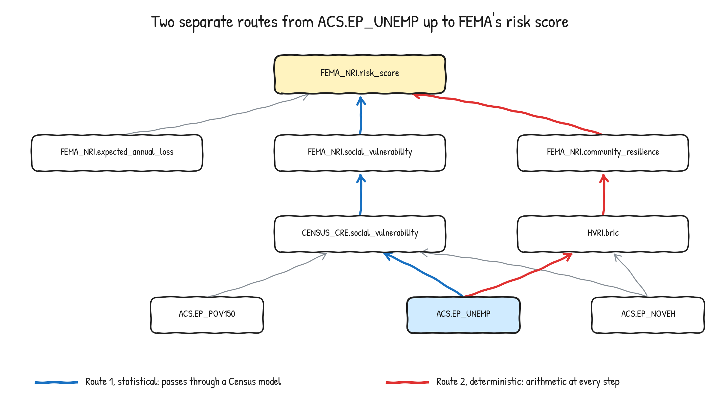
FEMA_NRI.risk_score and everything it was built from. Two routes, drawn in blue and red, both start at the same ACS unemployment column: one climbs through the Census Bureau’s resilience estimates, the other through HVRI’s BRIC index.

Suppose you want to predict the risk score using the poverty rate and the unemployment rate:

python3 mini_lint.py --target FEMA_NRI.risk_score --covariates ACS.EP_POV150 ACS.EP_UNEMP

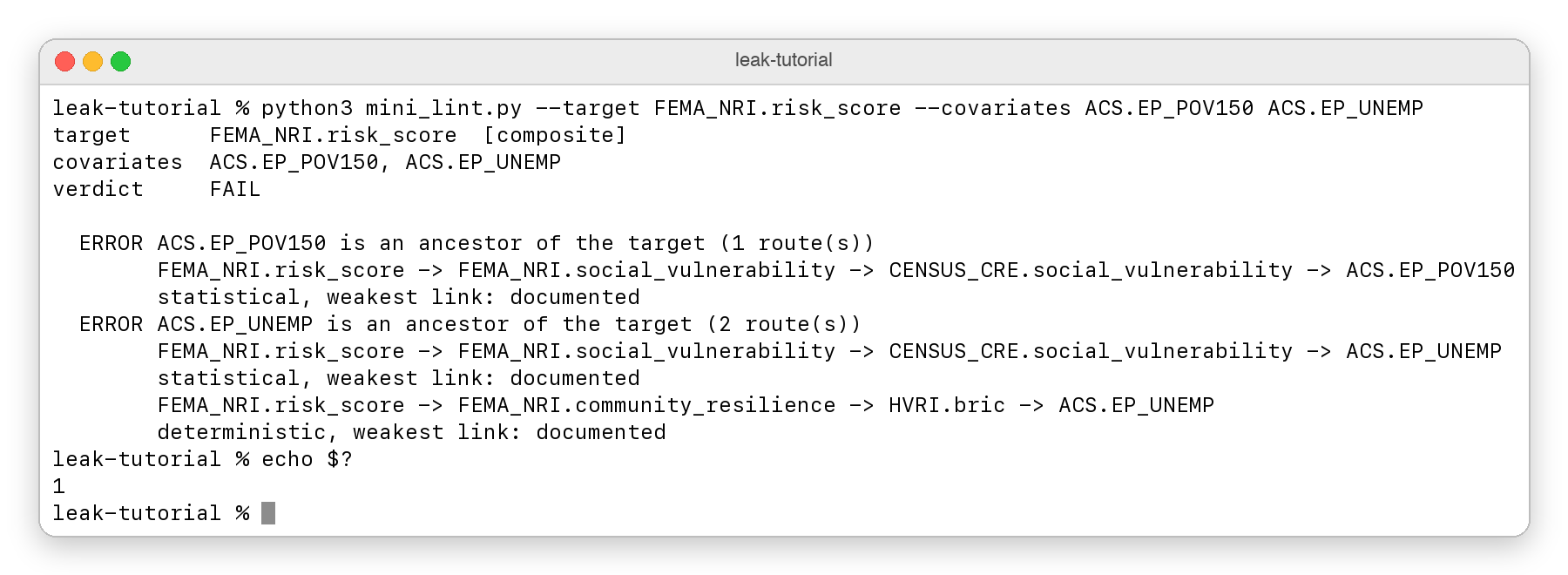
The verdict is FAIL. The poverty rate reaches the target by one route, and the unemployment rate reaches it by two, one statistical and one deterministic.

The verdict is FAIL, with exit code 1.

ACS.EP_POV150 reaches the target by one route. ACS.EP_UNEMP reaches it by two.

The first unemployment route passes through the Census model, so the tool labels it statistical. The second route passes through HVRI’s BRIC index, where unemployment is a direct ingredient, so the tool labels it deterministic.

Try tracing both routes by eye in a spreadsheet of column names and you’ll quickly see why a graph helps. The traversal finds both in a fraction of a second.

Case 2: A Descendant

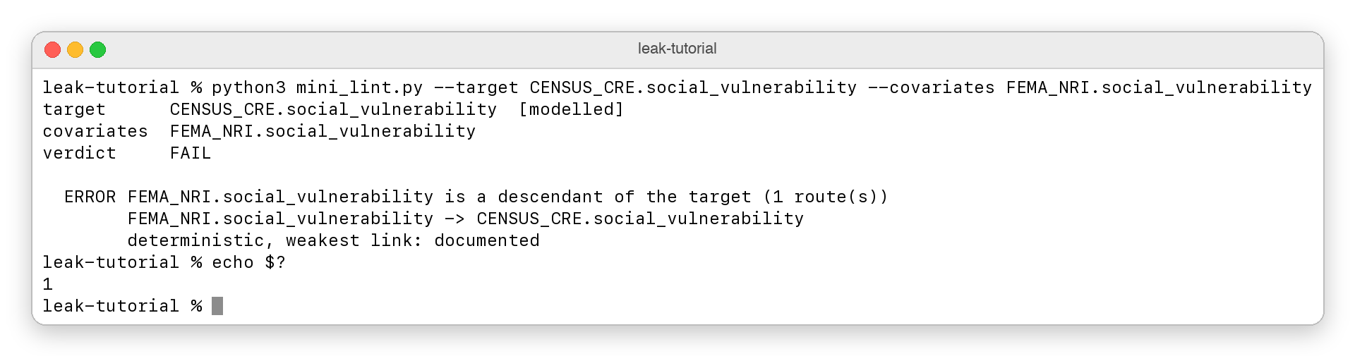
Now flip the direction and suppose you want to predict the Census score using FEMA’s republished copy of it as a covariate:

python3 mini_lint.py --target CENSUS_CRE.social_vulnerability --covariates FEMA_NRI.social_vulnerability

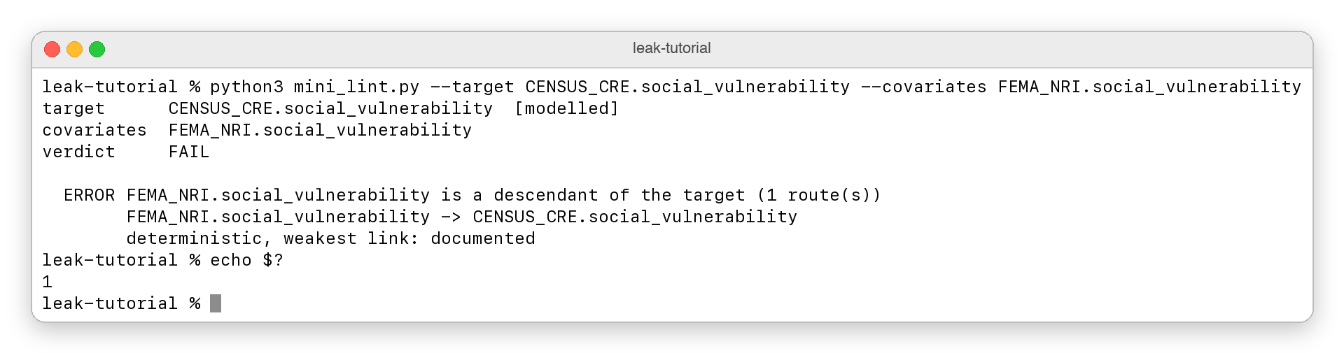
The flipped case, and another FAIL. FEMA’s republished copy of the Census score is a descendant of the target by one deterministic route.

FEMA’s score is built directly from the Census score, so using it as an input hands the model the answer. The tool catches this as a descendant.

Case 3: REVIEW, PASS, and UNTRACED

Here are three runs that should come back clean or nearly clean:

python3 mini_lint.py --target NVSS.mortality --covariates FEMA_NRI.social_vulnerability HVRI.bric
python3 mini_lint.py --target FEMA_NRI.risk_score --covariates SAT.chirps_rainfall
python3 mini_lint.py --target NVSS.mortality --covariates SAT.chirps_rainfall

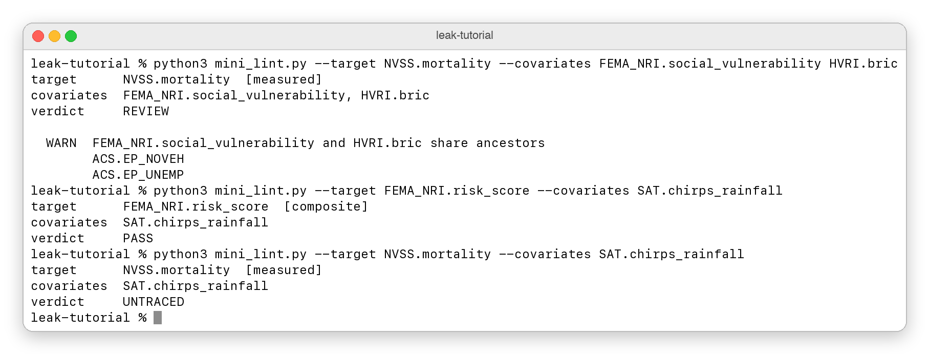
Three cleaner runs: REVIEW for the pair that shares two ACS parents, PASS for satellite rainfall against the risk score, and UNTRACED for a target with zero listed parents.

The first run returns REVIEW, because the two covariates share two ACS parents and overlap in what they tell the model.

The second run returns PASS, because the risk score has a traced family tree and satellite rainfall sits outside it.

The third run returns UNTRACED, because death certificate records are a direct count with zero listed parents.

These quiet results matter as much as the failures. A checker that raised an alarm on every input would be useless, so a good test set always includes cases that should pass.

Step 7: Make the Linter Fail Loudly on Bad Input

A safety tool earns trust by failing clearly. The worst outcome for a leak checker is a green PASS on a check that quietly skipped its work, and there are three common ways that can happen.

Trap 1: Typos in Names

To try this, copy mini-manifest.yaml to typo-manifest.yaml and change HVRI.bric to HVRI.brick inside the FEMA_NRI.community_resilience entry. Then run these two commands:

python3 mini_lint.py --target FEMA_NRI.risk_score --covariates ACS.EP_POV15
python3 mini_lint.py --manifest typo-manifest.yaml --target FEMA_NRI.risk_score --covariates ACS.EP_UNEMP

Two typos, two exit codes. The misspelled covariate becomes a FAIL with exit code 1, and the misspelled parent inside the manifest becomes a manifest error with exit code 2.

A misspelled covariate (ACS.EP_POV15) becomes a FAIL with exit code 1. A misspelled parent inside the manifest (HVRI.brick) becomes a manifest error with exit code 2. Both stop the run before any traversal happens.

Trap 2: Duplicate YAML Keys

Make another copy of the manifest called sneaky-manifest.yaml, then add one extra line at the very end of the file, inside the FEMA_NRI.risk_score block:

    derivesFrom: []

The risk score now has two derivesFrom keys. Create peek.py to see what plain PyYAML does with that:

import yaml

with open("sneaky-manifest.yaml") as fh:
    doc = yaml.safe_load(fh)

print(doc["products"]["FEMA_NRI.risk_score"]["derivesFrom"])

Now run peek.py, and then run the linter on the same file:

python3 peek.py
python3 mini_lint.py --manifest sneaky-manifest.yaml --target FEMA_NRI.risk_score --covariates ACS.EP_UNEMP

The duplicate key, seen two ways. Plain yaml.safe_load prints an empty list and says nothing, while the strict loader names the repeated key, both line numbers, and exits with code 2.

Plain yaml.safe_load returns an empty list, because PyYAML kept the second key, threw away all three real edges, and stayed silent about it. A linter built on that loader would find zero routes and let every leaky covariate through.

The strict loader stops with exit code 2 and points at both line numbers.

Trap 3: An Empty Covariate List

The third trap is easy to overlook. In CI, you might build the covariate list from a file or a shell variable. If that file is empty or the variable name has a typo, the command ends up with zero covariates.

An earlier version of my full tool accepted that and printed PASS, which is a clean bill of health for a check that skipped all its work.

python3 mini_lint.py --target FEMA_NRI.risk_score --covariates

An empty --covariates list now stops the run at argparse, before any traversal, with exit code 2.

In mini_lint.py, nargs="+" tells argparse that --covariates needs at least one value, and required=True makes the flag itself mandatory. An empty list now turns the pipeline red with exit code 2.

Step 8: Run the Check Automatically in CI

CI (continuous integration) runs checks for you every time you push code. This GitHub Actions workflow runs the linter on every push and every pull request. Save it as .github/workflows/lineage.yml in a repository that holds mini_lint.py and mini-manifest.yaml at its root:

name: lineage-check

on: [push, pull_request]

jobs:
  lint-lineage:
    runs-on: ubuntu-latest
    steps:
      - uses: actions/checkout@v5
      - uses: actions/setup-python@v6
        with:
          python-version: "3.12"
      - run: pip install pyyaml
      - name: Check covariates against the target's lineage
        run: |
          python3 mini_lint.py \
            --target FEMA_NRI.risk_score \
            --covariates $(cat features.txt)

Put your covariate names in a file called features.txt at the root of the repository, one name per line:

SAT.chirps_rainfall

The $(cat features.txt) part pastes those names into the command, and with this file the job passes and turns green. If someone later adds a leaky covariate such as ACS.EP_UNEMP, the job exits with code 1 and turns red. If someone empties features.txt by accident, argparse exits with code 2, and the job turns red as well.

exit code	meaning	CI result
0	the check ran and returned PASS, REVIEW, or UNTRACED	green
1	the check ran and found a leak	red
2	the manifest is broken or the command is malformed	red

REVIEW and UNTRACED also exit with code 0. If you want your pipeline to stop on those as well, change the last line of main so that every verdict other than PASS exits with code 1.

The companion repository runs this exact workflow, and you can see its results on the repository’s Actions tab.

Step 9: Learn from My Mistakes

Building the full manifest taught me that a linter is only as good as the graph it reads. I got the SVI wrong twice, in opposite directions, and both mistakes came from the same habit of trusting the columns in a file over the methodology behind it.

Mistake 1: The SVI California file contains 24 columns whose names start with EP_, but CDC ranks only 16 of them into the index. My first manifest counted all 24 and recorded EP_NOINT (broadband subscriptions) as an ingredient of the index. That column sits in the file, and CDC leaves it out of the ranking, so I removed the edge.

Mistake 2: I then over-corrected and listed all eight unranked columns as safe bystanders that ship beside the index. Seven of those eight are race and ethnicity columns. When I checked the raw counts, those seven added up to E_MINRTY exactly, and the largest difference across all 9,109 tracts was zero.

EP_MINRTY is the single input to Theme 3, and Theme 3 feeds the overall index.

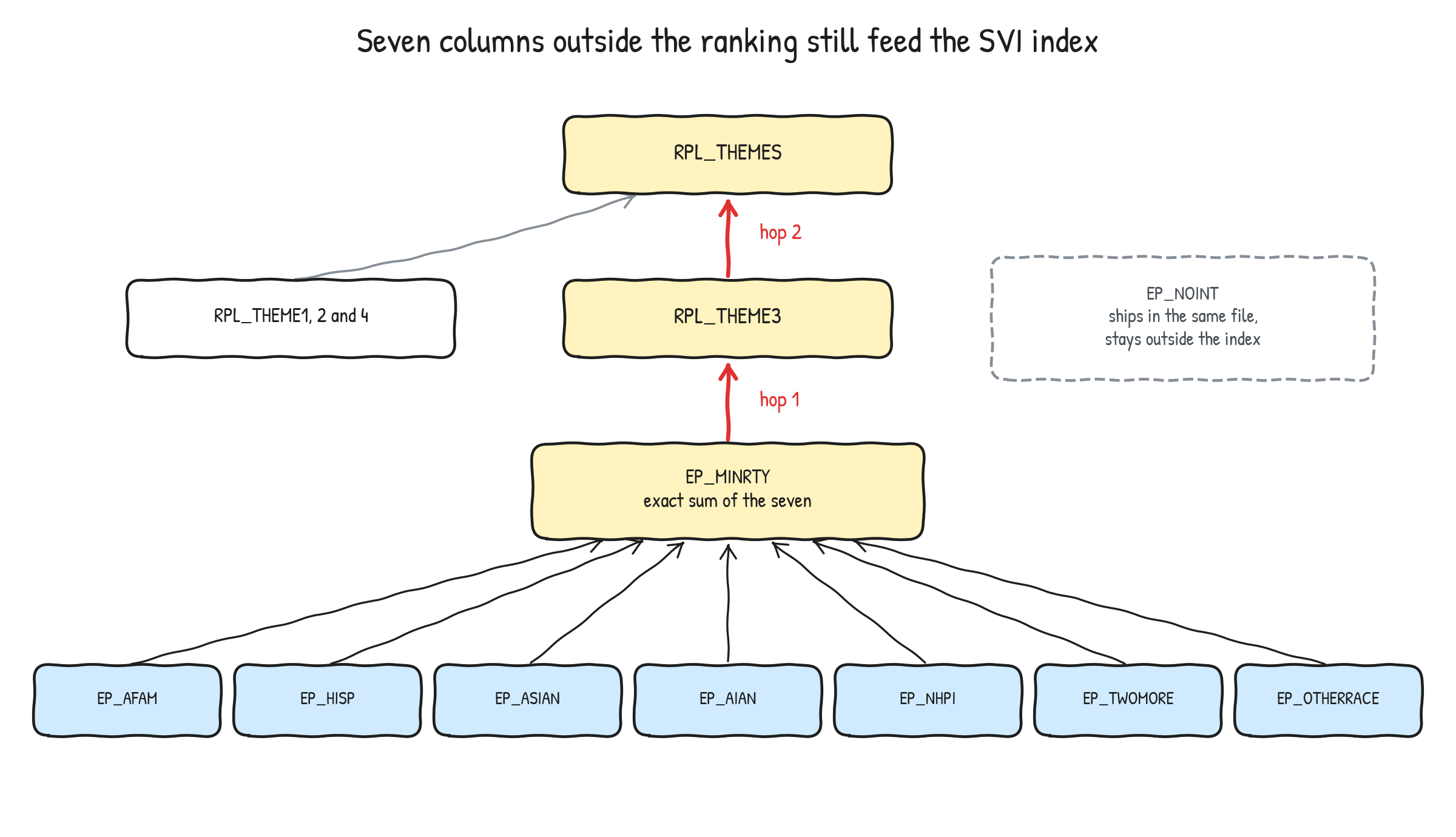
Why those seven columns aren’t bystanders. They sum exactly to EP_MINRTY, which feeds Theme 3 one hop up, which feeds the overall index one hop above that. EP_NOINT, in the dashed box, ships in the same file and stays outside the index.

So those seven columns are ancestors of the index, two hops up. My own linter had been clearing them as safe covariates for an SVI target, which is exactly the kind of false clearance the tool exists to prevent.

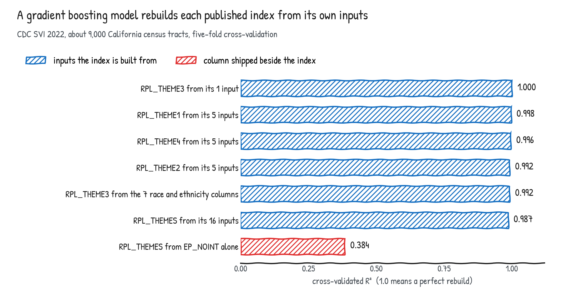
Cross-validated R² for each product, predicted from the columns listed beside it. Every product predicted from its own inputs scores 0.987 or higher, while EP_NOINT, which only ships beside the index, reaches 0.384.

The chart makes the difference plain: the seven race and ethnicity columns rebuild Theme 3 at R² = 0.992, while EP_NOINT alone reaches only 0.384 against the overall index.

I now follow a stricter rule before I mark any column as safe. I read the methodology first, and then I test the relationship in the data.

The full manifest records the result with a field called coPublishedNonInputs, which lists columns that ship in the same file as an index and take zero part in computing it. For the SVI, EP_NOINT is now the only entry.

The mini linter in this tutorial covers the core ideas. The full project adds:

• a manifest with 60 products and 75 derivation edges across US and global data, including CDC PLACES, FEMA’s National Risk Index, WorldPop, AlphaEarth satellite embeddings, and WFP’s HungerMap LIVE

• a written evidence note for every product that carries edges, plus a correction field wherever an earlier claim turned out to be wrong

• a --graph mode that prints the whole derivation graph

• a built-in suite of eight real audit cases

• a reproduce_svi.py script that checks every R² figure in this article against the live CDC file

• a pinned Dockerfile, so the figures reproduce exactly

To try it:

git clone https://github.com/Adeniyikayodee/dependency_manifest.git
cd dependency_manifest
python3 lint_lineage.py
python3 lint_lineage.py --graph
python3 reproduce_svi.py

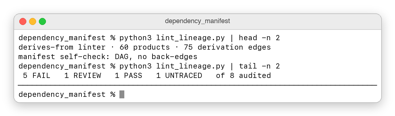
The full tool on the complete manifest: 60 products, 75 derivation edges, and eight audits that come back as 5 FAIL, 1 REVIEW, 1 PASS, and 1 UNTRACED.

The manifest is clear about its limits. It covers 60 products out of an estimated 400 or more official composite indices worldwide, and four of its edges are still marked inferred. The first audit of the file found six errors, and four of them sat in edges I had already labelled certain or documented.

The people best placed to write this kind of record are the agencies themselves, since they already describe their methods in PDF form. Two new fields on a public data schema, derivesFrom and measurementBasis, would give every producer a place to store what they already know.

If you work with public data, you can help by adding products you know well, or by checking the edges marked inferred against their source documents.

Conclusion

Target leakage in public data hides inside the recipes that agencies use to build their indices. A model can score close to perfect by rediscovering one of those recipes, and that score says very little about the real world.

In this tutorial, you:

• rebuilt CDC’s Theme 1 at R² = 0.998 from its own five input columns

• separated provenance (where a number arrived from) from derivation (what it was calculated from)

• wrote a YAML manifest that records derivation edges with a relation and a confidence level

• built a linter that uses breadth-first search to find ancestors and depth-first search to list every route

• made the linter fail loudly on typos, duplicate YAML keys, cycles, and empty covariate lists

• wired the check into GitHub Actions with clear exit codes

Before you trust a high score on public data, ask yourself what your target was built from. Once you write the answer down, a few lines of Python can check it every time you train a model.

The code from this tutorial lives in derives-from-tutorial, and you can find the full tool, the manifest, and the reproduction script in the main dependency_manifest repository. The project is archived on Zenodo with the DOI 10.5281/zenodo.22274757, and you are free to use it under the CC0 licence.

Sources